Non-Parametric Bootstrap in R With Correction for Bias and Skew

by Wyatt "Miller" Miller
Last revised March 14, 2018

Introduction

What Is the Non-Parametric Bootstrap Method in Statistics?

Non-parametric bootstrap is a resampling method that can provide insight into nearly any population statistic when the theoretical distribution of the statistic is complicated or unknown. The "magic" of bootstrapping presents itself when you have a single sample and cannot obtain more information about (or further samples from) the population of interest.

First published by Bradley Efron in "Bootstrap methods: another look at the jackknife" in 1979, the bootstrap methodology has seen improvement over the years, including a Bayesian extension developed in 1981[3]. The bias-corrected and accelerated (BCa) bootstrap was developed by Efron in 1987 and is demonstrated in a later section of this post.

Bootstrapping maintains a number of potent applications:

In machine learning (ML) and data science (DS), "bagging" (bootstrap aggregating) is an ensemble meta-algorithm designed to improve the stability and accuracy of machine learning algorithms used in statistical classification and regression that is based on the bootstrap methodology[1][9].
Bootstrapping can formulate confidence intervals from a population sample without requiring further information from the population of interest.
Bootstrapping can quickly estimate population statistics when samples are only obtainable in very small, but regularly recurring, subsets (e.g. big data feed samples in a live environment can be quickly estimated)
Bootstrapping can be used in time-series data, randomly censored data, and more[2].
The bootstrap method can estimate nearly any population statistic (e.g. mean, median, variance, etc.).

How Do Parametric and Non-Parametric Bootstrap Methods Differ?

Both parametric and non-parametric bootstrap are resampling methods that involve similar processes. Generally, these methods see the following differences[7]:

Parametric bootstrapping resamples from a known distribution (the parameters of which are estimated from the sample), while non-parametric bootstrapping resamples from the sample itself.
Parametric bootstrapping maintains an advantage over non-parametric bootstrapping when the sample size is very small (e.g. 10 observations) due to the smoothing effects offered by estimating the distribution.
Non-parametric bootstrapping tends to underestimate variance when performing confidence intervals due to the jagged shape and bounds of the distribution; parametric bootstrapping is more accurate with confidence interval variance estimation, but only if the correct distribution model has been ascertained from the sample.
While the power of the parametric bootstrap method can be higher than that of the non-parametric method, the parametric method is completely dependent on choosing the correct distribution model (and parameters) from the given sample; verifying the accuracy of the chosen model may be impossible if the population is inaccessible for further testing. It is this dependency that has determined why this article is pursuing a non-parametric bootstrap versus a parametric bootstrap method.

How Do the Sample, Sampling, and Bootstrap Distributions Differ?

Throughout this article, it is assumed the population is large (or infinite).

Recall the sample distribution simply requires a single, large enough (truly random) sample from a population. If this sample is truly "large enough" (which is generally quite large), it will converge in probability to the population - a necessary sample size can be computed if the population size is known. Thus conjectures about said population can be made directly from the distribution of the sample collected. Often this large of a sample is unobtainable, which is what is assumed in this article, hence the need for either the sampling distribution or bootstrapping.

The sampling distribution is the distribution of a chosen statistic from many samples of a population. To calculate the sample distribution:

A desired statistic for a population is chosen.
A sample is drawn from the population of size n with replacement, large enough to satisfy the Central Limit Theorem (approximately 30 to 50 or more).
The statistic for that sample is computed and recorded.
All samples are drawn from the population, their statistics computed and recorded.
The aggregate sampling information is used to formulate the sampling distribution, which will be normally distributed.

Key differences between the sampling distribution and bootstrap methods include:

To formulate the true theoretical sampling distribution, all of the population must be accessible (which negates the need for any of these methods); otherwise, the sampling distribution can be estimated with a large number of samples.
The sampling distribution likely requires further access to the population, while bootstrap methods do not.
Bootstrap methods assume the population of interest is well-represented in the sample being examined; the sampling distribution does not directly assume this, but does assume proper randomization.
The sampling distribution assumes a sample size large enough to satisfy the Central Limit Theorem, while the bootstrap methods rely only on the assumption that the sample is representative of the population.
Both methods assume proper sample randomization and independence among observations.
Both methods can estimate a wide variety of statistics (e.g. mean, median, variance, etc.)

In short, the sampling distribution is useful if the population of interest can be accessed for more information (e.g. campus surveys), while bootstrapping methods are more useful when only a single sample is present, which is not large enough to infer about the population, but representative of the population (e.g. randomized blood draw data from patients with a rare disease).

Assumptions of Bootstrapping Methods

Bootstrap methods assume the following[8]:

Independence among the observations sampled from the population of interest.
True random selection when the sample is collected from the population.
A population of sufficient magnitude (infinite or sufficiently large).
The sample and its distribution are a good approximation of the population and its distribution (the sample is representative of the population).
Possible other assumptions native to the statistic of interest or the distribution being used in the case of parametric bootstrapping.

How it Works

How Is an Non-Parametric Bootstrap Computed?

The non-parametric bootstrap (more simply "bootstrap" from here on) is computed through the following process:

A desired test statistic for a population is chosen.
A random sample of a population is obtained - a preliminary decision can made as to whether or not this sample is representative of the population.
The sample is resampled using the same size sample with replacement.
The test statistic for that resample is computed and recorded.
A large number of these resamples are drawn, their statistics computed and recorded.
The aggregate resample information is used to formulate the bootstrap distribution.

Resampling with replacement is the cornerstone of the bootstrap process. For example, let's assume you wish to know the average age of students on a certain college campus. Assume you are able to query six students (randomly) throughout the campus and obtain the following set {19, 24, 18, 18, 21, 19}. You believe this to be representative of the population, so you decide to begin the bootstrap process. On the first iteration of the bootstrap, this original sample is resampled randomly with replacement (e.g. {18, 21, 18, 21, 24, 24}) and the test statistic is computed (21) and recorded. The original sample is resampled with replacement again, the test statistic again is computed and recorded. This process occurs a large number of times, generating the bootstrap distribution from which confidence intervals are created to ascertain the true test statistic of the population (in this case, the true population mean of students' age on campus).

Observe that the sample size is concerningly small in the example above, however it is believed to be representative of the population. If this assumption cannot be made, possible options to increase the power of the bootstrap process include:

Perform a parametric bootstrap instead, which tends to have more power than a non-parametric bootstrap, but requires the bootstrap estimated distribution function to be representative of the population.
Gather more random queries from the population of students.

Applied Analysis

Bootstrap from the Ground Up

In the following code, the bootstrap distribution of a gamma-distributed population is computed in R. The chosen test statistic is the mean.

Data on an entire population is often not available, hence the need for sampling in the first place. In the following scripts, the populations of interest are pre-generated, allowing the results to be compared. It is easy to pretend, however, that the process begins at sample collection.

NOTE: Setting the seed is not required - it will simply duplicate the results discussed below.

set.seed(585)
my.population <- rgamma(100000, 2, 2)
my.sample <- sample(my.population, size=30)

my.bootstrap <- numeric(5000)
for(i in 1:length(my.bootstrap)) {
  my.bootstrap[i] <- mean(sample(my.sample, replace=TRUE))
}

quantile(my.bootstrap,0.025)
quantile(my.bootstrap,0.975)

The code above begins by creating a large population of interest (100,000 observations). It then selects a random sample of size 30; this is where studies would likely start the statistical process. A numeric vector is created to capture the bootstrap test statistic computations (the mean in this case) and the primary for-loop begins. In each iteration, the sample is resampled (of the same size, 30) with replacement, and the mean of this resample is computed and captured. This is performed a large number of times (5,000 iterations). After the loop concludes, quantile functions are applied to determine the inner 95th percentile of the bootstrap distribution - with the given seed, this interval is approximately 0.868 to 1.642.

A comparative histogram is quick way to visualize this interval visual method:

hist(my.population, freq=FALSE, ylim=c(0,1), breaks=48)
abline(v=mean(my.population), lty=1, lwd=2, col="blue")
abline(v=mean(my.bootstrap), lty=1, lwd=2, col="red")
abline(v=quantile(my.bootstrap,0.975), lty=2, lwd=1, col="red")
abline(v=quantile(my.bootstrap,0.025), lty=2, lwd=1, col="red")

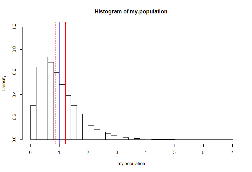
Observe the true average population mean (blue) falls within the 95% confidence interval of this bootstrap distribution as desired. Despite this success, this should not yet be considered an applied validation of the bootstrap process.

Validating the Results (Monte Carlo)

WARNING: This process can be time consuming on slower computers.

In the example above, the confidence interval indicates with 95% certainty that the true population mean falls between approximately 0.868 and 1.642; accurate in this case since the true population mean is 1, which falls within the confidence bands.

To confirm these results (at least from an applied perspective), the bootstrap process can be run a large number of times to determine how often it is accurate:

set.seed(585)
bootstrap.success.95 <- 0
shape.parameter <- seq(1, 9, by=0.25)
scale.parameter <- seq(1, 2, by=0.25)

for (i in 1:4000) {
  my.population <- rgamma(100000, sample(shape.parameter, 1), sample(scale.parameter, 1))
  my.sample <- sample(my.population, size = sample(100:500, 1))
  
  my.bootstrap <- numeric(5000)
  for(i in 1:length(my.bootstrap)) {
    my.bootstrap[i] <- mean(sample(my.sample, replace=TRUE))
  }
  
  if ((quantile(my.bootstrap,0.025)<=mean(my.population)) & (mean(my.population)<=quantile(my.bootstrap, 0.975))) {
    bootstrap.success.95 <- bootstrap.success.95+1
  }
}

(bootstrap.success.95/4000)

To offer broader results in the above code, the gamma distribution shape and scale are randomized among quarter intervals along appropriate domains. The sample size is also randomized in integers from 100 to 500. The bootstrap method is performed 4,000 times and the ratio of successful confidence intervals is printed.

With this seed, the proportion of correct confidence interval predictions falls at approximately 94.725%. While this is close to the desired 95%, it may be distressing to the rigorous statistician that their confidence intervals maintain such error. There are a number of explanations for this behavior:

Recall that the bootstrap sample assumes the sample is a good approximation of the population[4]. In most of the randomized gamma distributions above there is heavy skew. Since the sample distribution is always symmetric, it is not a good representation of the population. Choosing a distribution that is more well-represented by its sample distribution (e.g. a Normal distribution) would improve results.
Bias, error, and skew have not been corrected for. Manually computing these measures is beyond the scope of this article, however it should be noted that both bias and standard error can be quickly computed from member variables of the boot() object seen below[5].

Leveraged Analysis

Accounting for Bias and Skew

Manually computing bias (a correction for the measure of center) and acceleration (a correction for skew) is beyond the scope of this article. However, there exist libraries and tools which can be easily leveraged to perform these tasks. This section leverages the "boot" library and "boot.ci" functions. First, install the library by running the following line in the R console:

install.packages("boot", dep=TRUE)

Now, consider the following script:

library(boot)

stat_fx <- function(s, i){ return(mean(s[i])) }

set.seed(585)
my.population <- rgamma(100000, 2, 2)
my.sample <- sample(my.population, size=30)
my.bootstrap <- boot(my.sample, stat_fx, R=5000)

boot.ci(my.bootstrap, type="bca")

hist(my.population, freq=FALSE, ylim=c(0,1), breaks=48)
abline(v=mean(my.population), lty=1, lwd=2, col="blue")
abline(v=my.bootstrap$t0[1], lty=1, lwd=2, col="red")
abline(v=boot.ci(my.bootstrap, type="bca")$bca[4:5], lty=2, lwd=1, col="red")

While the above code isn't much more concise than the manually computed version in the previous section, it provides a "Bias Corrected and Accelerated" (BCa) confidence interval which accounts for both bias and skew (aka. "accelerated" confidence interval). The goal of BCa is to "automatically create confidence intervals that adjust for underlying higher order effects."[6] Note that the upper- and lower-bounds of the confidence intervals in the two histograms above are slightly different due to correction.

Again we show a successful singleton estimate of the population mean, estimated to be between 0.900 and 1.695 after correction.

Validating the Results (Monte Carlo)

WARNING: This process can be time consuming on slower computers.

As above, the results of this analysis can be validated (from an applied perspective) through iterative analysis and randomization of inputs:

library(boot)

stat_fx <- function(s, i){ return(mean(s[i])) }

set.seed(585)
bootstrap.success.95 <- 0
shape.parameter <- seq(1, 9, by=0.25)
scale.parameter <- seq(1, 2, by=0.25)

for (i in 1:4000) {
  my.population <- rgamma(100000, sample(shape.parameter, 1), sample(scale.parameter, 1))
  my.sample <- sample(my.population, size = sample(100:500, 1))
  my.bootstrap <- boot(my.sample, stat_fx, R=5000)
  
  if ((boot.ci(my.bootstrap, type="bca")$bca[4]<=mean(my.population)) & (mean(my.population)<=boot.ci(my.bootstrap, type="bca")$bca[5])) {
    bootstrap.success.95 <- bootstrap.success.95+1
  }
}
(bootstrap.success.95/4000)

This computation consistently produces successful confidence intervals approximately 94.975% percent of the time, a more desirable result than the uncorrected confidence interval above.

Further Considerations

The Test Statistic Function

As noted above, the bootstrap method can work on most any test statistic. In the majority of cases, simply changing the static function to produce the desired statistic is sufficient. For example, to find the median instead of the mean:

stat_fx <- function(s, i){
   return(median(s[i]))
}

Confidence Interval Type

The boost library has five confidence interval types available:

The normal approximation method
The basic bootstrap method (demonstrated above, computed manually)
The studentized bootstrap method
The bootstrap percentile method
The bias corrected and accelerated (BCa) method (demonstrated above)

To access the other interval types a vector of selected types can be provided, or the "type=" parameter can be omitted entirely to select all options:

boot.ci(boot.out=my.bootstrap)
boot.ci(boot.out=my.bootstrap, type=c("norm", "basic", "stud", "perc", "bca"))

The above two lines of code will produce the same output.

NOTE: To produce confidence intervals using the studentized bootstrap method, bootstrap variance must be computed in the test statistic function.

To compute the variance for the studentized bootstrap method, the following modification can be made to the test statistic function:

stat_fx <- function(s, i){
   return(c(mean(s[i]), var(s[i])/length(i)))
}

Confidence Level

It may be desirable to change the confidence level of your bootstrap procedure; the default option (95%) is used in the code above. Examples of further options are shown below:

boot.ci(boot.out = my.bootstrap, conf=0.90)
boot.ci(boot.out = my.bootstrap, conf=0.95)
boot.ci(boot.out = my.bootstrap, conf=0.99)

Population Distributions

The following are several replacement examples for the gamma-distributed population presented above:

my.population <- rbinom(100000, 5, 0.2)
my.population <- rpois(100000, 2)
my.population <- rchisq(100000, 2)
my.population <- rexp(100000, 2)
my.population <- rnorm(100000, 0, 1)
my.population <- rt(100000, 2)
my.population <- runif(100000, 0, 2)

A Quick Note on Sample Size...

The bootstrap distribution is a powerful estimator of population statistics, even with very low sample sizes (e.g. 10). The above code which leverages the boot library was able to formulate accurate confidence intervals approximately 89% of the time.

Final Thoughts

Things to Consider

While the confidence intervals from the manual computation and the library-based computation ("basic" confidence interval type in the boot.ci() output) are similar, they do not match despite setting the same random seed. This is likely due to the method that the boot library uses to choose its sample: it is probably not based on the sample() function as performed in the manual computation.
Achieving a true 95% confidence using the above scripts is difficult unless you are working with a friendly, symmetric distribution (which is unlikely outside of an experimental environment). This was the primary impetus for using gamma-distributed population data above: to introduce heavy skew and bias which cannot fully be accounted for. While the script which leverages the boot library comes closer to the desired 95% prediction rate, it still falls a bit shy.
Bootstrapping is only as powerful as the sample provided. If a sample is not truly randomized from the population, the sample will tend toward a subset of the population rather than the population as a whole. This tendency can overpower bias correction, eliminating the validity of any confidence intervals. Proper randomization of the sample is crucial.
As mentioned several times throughout this article, the validity of a bootstrap confidence interval is highly dependent on the assumption that the sample distribution is a representative approximation of the population.